Correlations, seasonality, lift and CUPED

Introduction

This is the fourth post about CUPED. The previous three were:

• Reducing variance in A/B testing with CUPED
• Reducing variance in conversion A/B testing with CUPED
• A/A testing and false positives with CUPED

In this final post, I will address some questions relating to CUPED:

• what if some units are missing "before" data?
• what if "before" and "after" is not correlated?
• what if "before" and "after" is correlated, but the treatment lift is 0?
• what if our measurement is not continuous (like USD spend per user), but binary conversion data?
• what if we run an A/B test, and evaluate using both traditional and CUPED methodology, and pick the "more favorable"?
• is correlation between "before" and "after" the same as seasonality?
• what are other ways to reduce variance in A/B testing?

What if some units are missing "before" data?

With CUPED, we can reduce the variance of our A/B test measurement, assuming we have "before" data, and it is correlated with the data collected during the experiment, which I referred to as "after" data in the last posts. But what if for some experimental units, the "before" data is missing? For example, we can imagine that the experiment unit is users, and for some users, we are missing the "before" data. In this case, all we have to do is: use the un-adjusted "after" metric. So, including this modification in the "CUPED recipe" from the first post:

Let $Y_i$ be the ith user's spend in the "after" period, and $X_i$ be their spend in the "before" period, both for A and B combined. We compute an adjusted "after" spend $Y'_i$ with the following process:

1. Compute the covariance $cov(X, Y)$ of X and Y.
2. Compute the variance $var(X)$ of X.
3. Compute the mean $\mu_X$ of X.
4. For the i'th user, if $X_i$ is missing: $ Y'_i := Y_i $.
5. For the i'th user, if $X_i$ is not missing:$ Y'_i := Y_i - (X_i - \mu_X) \frac{cov(X, Y)}{var(X)} $.
6. Evaluate the A/B test using $Y'$ instead of $Y$.

What if "before" and "after" are not correlated?

If "before" and "after" are not correlated, and we use CUPED, are we making a mistake? No. This question was answered in the first first post. If there is no correlation, then in the above equation $ cov(X, Y) = 0 $, so $ Y_i' = Y_i $. In actual experiment instances $ cov(X, Y) $ will not be exactly 0, but will be a small number, so $ cov(X, Y) \approx 0 $, so $ Y_i' \approx Y_i $. Running Monte Carlo simulations of many experiments showed that over many experiments this is equivalent to traditional A/B testing.

What if "before" and "after" is correlated, but the treatment lift is 0?

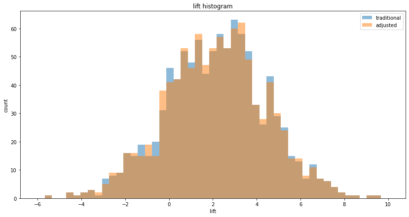
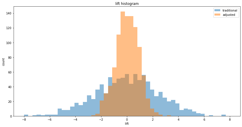
This was explored in the third post. If the treatment lift is 0, then in an A/B test the null hypothesis is actually true, and we're really running an A/A test. In this case, we still get the benefit of CUPED, we're just getting a more reliable measurement of the 0 lift. CUPED doesn't care what the lift is, it reduces the variance of the lift measurement in all cases, if there is correlation. See the plot below of an A/A test, where the variance is reduced for 0 lift (the histogram is centered on 0):

What if our measurement is not continuous, but binary conversion data?

This was explored in the second post for the binary 0/1 conversion case, and it is not a problem, CUPED can be applied. But it is somewhat counter-intuitive, since the CUPED-adjusted values are no longer 0 and 1, but become continuous. Since the CUPED formula has 2 variables, before and after, and in the binary case each can take on the value 0 and 1, there are 4 possible CUPED-adjusted values. In one experiment realization from that post, these values were:

Possible mappings:
(before=1, after=0) -> adjusted=-0.722
(before=0, after=1) -> adjusted=1.081
(before=0, after=0) -> adjusted=0.081
(before=1, after=1) -> adjusted=0.278

This illustrates that the binary data loses its binary nature with CUPED.

What if we run an A/B test, and pick the "more favorable" outcome?

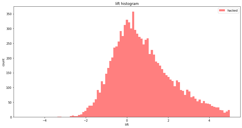
What if we run an A/B test, evaluate using both traditional (without using "before" data) and CUPED A/B testing, and pick the more favorable outcome, the one with higher lift / lower p-value? This was explored in the third post, and was shown to be a fallacy. We showed with Monte Carlo simulations that this behavior skews the lift distribution to the right and overestimates the lift:

Note that this error is similar to other "p-hacking" fallacies:

• peeking at experiment results before the experiment finishes (and stopping early in case of favorable results)...
• evaluating multiple metrics (and using the most favorable one to report results)...
• checking multiple subsets like countries for favorable results...

... without controlling the p-value for multiple checks.

Is correlation between "before" and "after" the same as seasonality?

No, they are different things. In the first post, I used this toy model to generate correlated "before" and "after" data:

def get_AB_samples(before_mean, before_sigma, eps_sigma, treatment_lift, N):
    A_before = list(normal(loc=before_mean, scale=before_sigma, size=N))
    B_before = list(normal(loc=before_mean, scale=before_sigma, size=N))
    A_after  = [x + normal(loc=0, scale=eps_sigma)                  for x in A_before]
    B_after  = [x + normal(loc=0, scale=eps_sigma) + treatment_lift for x in B_before]
    return A_before, B_before, A_after, B_after

Notice that here, A_before and A_after both have the same mean, before_mean, since A_after is just A_before with some (symmetric) noise added (the same is true for the Bs if treatment_lift = 0). So here we have a correlated experiment, but the means are the same before and after, there is no seasonal change. Now look at this:

def get_AB_samples(before_mean, before_sigma, seasonal_lift, treatment_lift, N):
    A_before = list(normal(loc=before_mean, scale=before_sigma, size=N))
    B_before = list(normal(loc=before_mean, scale=before_sigma, size=N))
    A_after  = list(normal(loc=before_mean + seasonal_lift                   scale=before_sigma, size=N))
    B_after  = list(normal(loc=before_mean + seasonal_lift + treatment_lift, scale=before_sigma, size=N))
    return A_before, B_before, A_after, B_after

In this setup, A_after has a seasonal_lift compared to A_before (and B has an optional treatment_lift), but A and B are uncorrelated.

These examples show that seasonality and correlation are not the same thing in A/B testing. Seasonality is a shift in the mean between before and after, correlation is correlation. All 9 combinations between {no correlation, correlation} x {no seasonal lift, seasonal lift} x {no treatment lift, treatment lift} are possible and occur in real life. CUPED only helps in reducing variabce if there is correlation.

What are other ways to reduce the variance of the lift measurement?

In these Monte Carlo simulations, I used the difference in means for lift:

def lift(A, B):
    return mean(B) - mean(A)

Because of the Central Limit Theorem, the distribution of the error of the mean measurement is a normal, and the difference of two normals is also normal. This is the bell curve we've been seeing on all the Monte Carlo histograms. The standard deviation of this normal is called the standard error, and its formula is $ s = \frac{\sigma}{\sqrt{N}} $. The important part here is the $ \sqrt{N} $, which says that for every 4x sample size, variance of the lift goes down 2x. So, another way to reduce variance of the lift measurements is to collect more N samples, if possible.

The other important method for reducing variance is stratification, where we identify sub-populations of our overall population and calibrate our sampling accordingly, or re-weight sub-population metrics after sampling.

Conclusion

This is the fourth and final post on CUPED. In the future I plan to write about stratification, another method to reduce variance in A/B testing.