Early stopping in A/B testing
Marton Trencseni - Thu 05 March 2020 - Data
Introduction
In the past posts we’ve been computing p values for various frequentist statistical tests that are useful for A/B testing (Z-test, t-test, Chi-squared, Fisher's exact). When we modeled the A/B test, we assumed the protocol is:
- decide what metric we will use to evaluate the test (eg. conversion, timespent, DAU)
- dedice how many $N$ samples we will collect
- decide what type of test (eg. t-test or $\chi^2$) we will use
- decide $\alpha$ acceptable false positive rate (FPR)
- collect $N$ samples
- compute $p$ value, if $p < \alpha$ reject the null hypothesis, else accept it
The code shown below is up on Github.
Early stopping
What happens if the tester is curious or impatient and follows a different protocol and peeks at the data repeatedly to see if it’s “already significant”. So instead of steps 5-6 above, they:
- collect $N_1$ samples, run hypothesis test on $N’ := N_1$ samples, compute $p$ value, if $p < \alpha$ reject the null hypothesis and stop, else go on
- collect $N_2$ more samples, run hypothesis test on $N’ := N + N_2$ samples, compute $p$ value, if $p < \alpha$ reject the null hypothesis and stop, else go on
- collect $N_3$ more samples...
- stop if $N’ >= N$
We can simulate this early stopping protocol with Monte Carlo code:
def abtest_episode(funnels, N, prior_observations=None):
    observations = simulate_abtest(funnels, N)
    if prior_observations is not None:
        observations += prior_observations
    p = chi2_contingency(observations, correction=False)[1]
    return observations, p

def early_stopping_simulation(funnels, num_simulations, episodes, alphas):
    hits = 0
    for _ in range(num_simulations):
        observations = None
        for i in range(len(episodes)):
            observations, p = abtest_episode(funnels, episodes[i], observations)
            if p <= alphas[i]:
                hits += 1
                break
    p = hits / num_simulations
    return p
Let’s assume our A/B test is actually not working (no lift), so both A and B are the same:
funnels = [
    [[0.50, 0.50], 0.5], # the first vector is the actual outcomes,
    [[0.50, 0.50], 0.5], # the second is the traffic split
]
First, let’s check that we get what we expect in the simple case, without early stopping:
Ns = [3000]
alphas = [0.05]

p = early_stopping_simulation(funnels, T, Ns, alphas)
print('False positive ratio: %.3f' % p)
Prints something like:
False positive ratio: 0.057
This is what we expect. If the null hypothesis is true (A and B are the same), we expect to get $\alpha$ false positives, that’s exactly what $\alpha$ controls. Let’s see what happens if we collect the same amount of total samples, but follow the early stopping protocol with 2 extra peeks:
Ns = [1000] * 3
alphas = [0.05] * 3

p = early_stopping_simulation(funnels, T, Ns, alphas)
print('False positive ratio: %.3f' % p)
Prints something like:
False positive ratio: 0.105
This is the problem with early stopping! If we repeatedly perform the significance test at the same $\alpha$ level, the overall $\alpha$ level will be higher. If we do this, we will on average have a higher false positive rate than we think. In the above simulation, with 2 extra peeks, at equal $N$ intervals, the FPR roughly doubles!
Intuition
Why does the FPR go up in the case of early stopping? The best way to see this is to evaluate the $p$ value a lot of times, and plot the results. The simulation code is straightforward:
def repeated_significances(funnels, episodes):
    results = []
    observations = None
    for i in range(len(episodes)):
        observations, p = abtest_episode(funnels, episodes[i], observations)
        N = np.sum(observations)
        results.append((N, p))
    return results
Let’s evaluate at every 100 samples, 100 times (total $N=10,000$), and run it 3 times:
Ns = [100] * 100

results1 = repeated_significances(funnels, Ns)
results2 = repeated_significances(funnels, Ns)
results3 = repeated_significances(funnels, Ns)

plt.figure(figsize=(10,5))
plt.xlabel('sample size')
plt.ylabel('p')
plt.plot([x[0] for x in results1], [x[1] for x in results1])
plt.plot([x[0] for x in results2], [x[1] for x in results2])
plt.plot([x[0] for x in results3], [x[1] for x in results3])
plt.plot([x[0] for x in results3], [0.05 for _ in results3])
plt.legend(['Test 1', 'Test 2', 'Test 3', 'p = 0.05'], loc='upper right')
plt.show()
The result is something like:
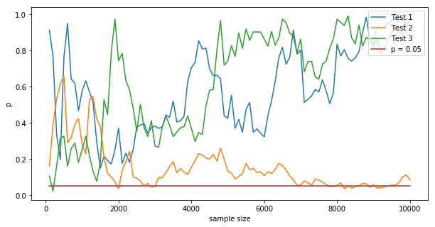
There is no “correct” $p$ value to compute at any point, since we are collecting samples from random process. The guarantee of frequentist hypothesis testing (as discussed in the past posts), is that, if we evaluate the data at the end (at $N=10,000$ on the chart, at the end), if the null hypothesis is true, then on average in $1-\alpha$ fraction of cases the p value will be bigger than $\alpha$, and we will make the correct decision to accept the null hypothesis (the correct decision). But there is no guarantee about the trajectory of the p value in between. The trajectory is by definition random, so if we repeatedly test against the $p=0.05$ line with an early stopping protocol, then we will reject the null hypothesis (the incorrect decision) more often. In the case above, for the green line, we would have done so at the beinning, and for the orange line, we could have done so several times; even though at the end, as it happens, these tests would all (correctly) accept the null hypothesis.
A mathy way of saying this is to realize that $P(p_{N} < \alpha | H_0)$ < $P(p_{N1} < \alpha | H_0) + P(p_{N1+N2} < \alpha | H_0 \wedge p_{N1} > \alpha)) + ...$
Alpha spending in sequential trials
In itself, an early stopping protocol is not a problem. In the above example, we saw that taking 2 extra peeks at equal $N$ intervals with early stopping at $\alpha=0.05$ each yields an overall $\alpha$ of ~0.10. As long as we know that the overall $\alpha$ of our protocol is what it is, we’re fine. The problem is if we’re not aware of this, and we believe we’re actually operating at a lower $\alpha$, and potentially report a lower $\alpha$ along with the results.
What if we are mindful of the increase in $\alpha$ that early stopping induces, but we want to keep the overall (=real) $\alpha$ at a certain level, let’s say $\alpha=0.05$. Based on the previous simulation, intuitively, this is possible, we just have to test at lower $\alpha$ at each early stopping opportunity. This is called alpha spending, because it’s like we have an overall budget of $\alpha$, and we’re spending it in steps. Note that alpha spending is not additive! Let’s look at two protocols to achieve overall $\alpha=0.05$.
First, the Pocock boundary, from Wikipedia:
The Pocock boundary gives a p-value threshold for each interim analysis which guides the data monitoring committee on whether to stop the trial. The boundary used depends on the number of interim analyses.
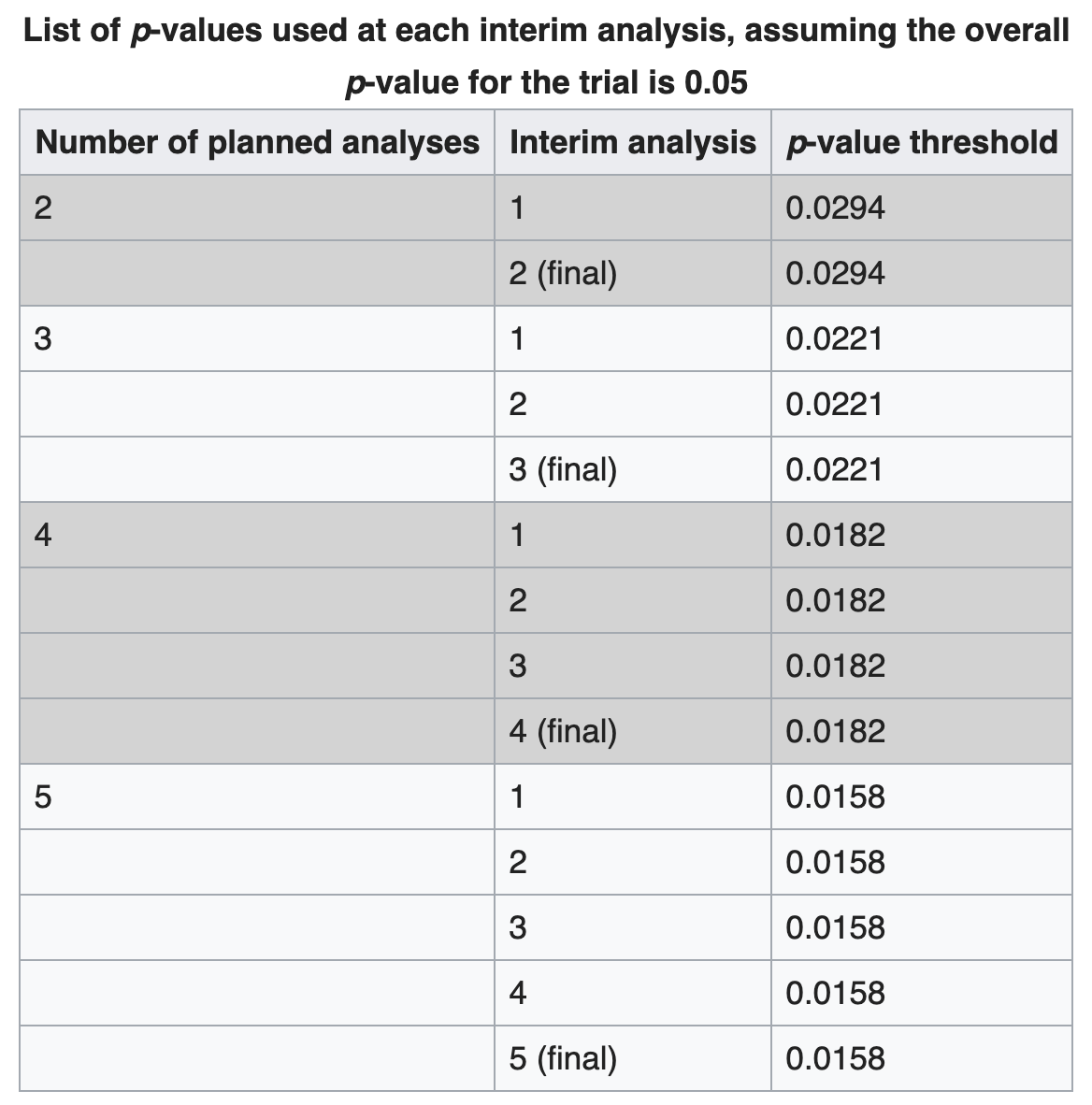
The Pocock boundary is simple to use in that the p-value threshold is the same at each interim analysis. The disadvantages are that the number of interim analyses must be fixed at the start and it is not possible under this scheme to add analyses after the trial has started. Another disadvantage is that investigators and readers frequently do not understand how the p-values are reported: for example, if there are five interim analyses planned, but the trial is stopped after the third interim analysis because the p-value was 0.01, then the overall p-value for the trial is still reported as <0.05 and not as 0.01.
So, in the simulated case earlier, if we use $\alpha=0.0221$ at each step, we will achieve an overall $\alpha=0.05$:
Ns = [1000] * 3
alphas = [0.0221] * 3

p = early_stopping_simulation(funnels, T, Ns, alphas)
print('False positive ratio: %.3f' % p)
Prints something like:
False positive ratio: 0.052
It works!
The Haybittle–Peto boundary is much simpler, but it’s not an exact rule. It essentially says, perform the in-between tests at a very low $\alpha=0.001$, and the final test at the desired $\alpha=0.05$. Because the the early steps were performed at such low $\alpha$, it doesn’t change the overall $\alpha$ by much.
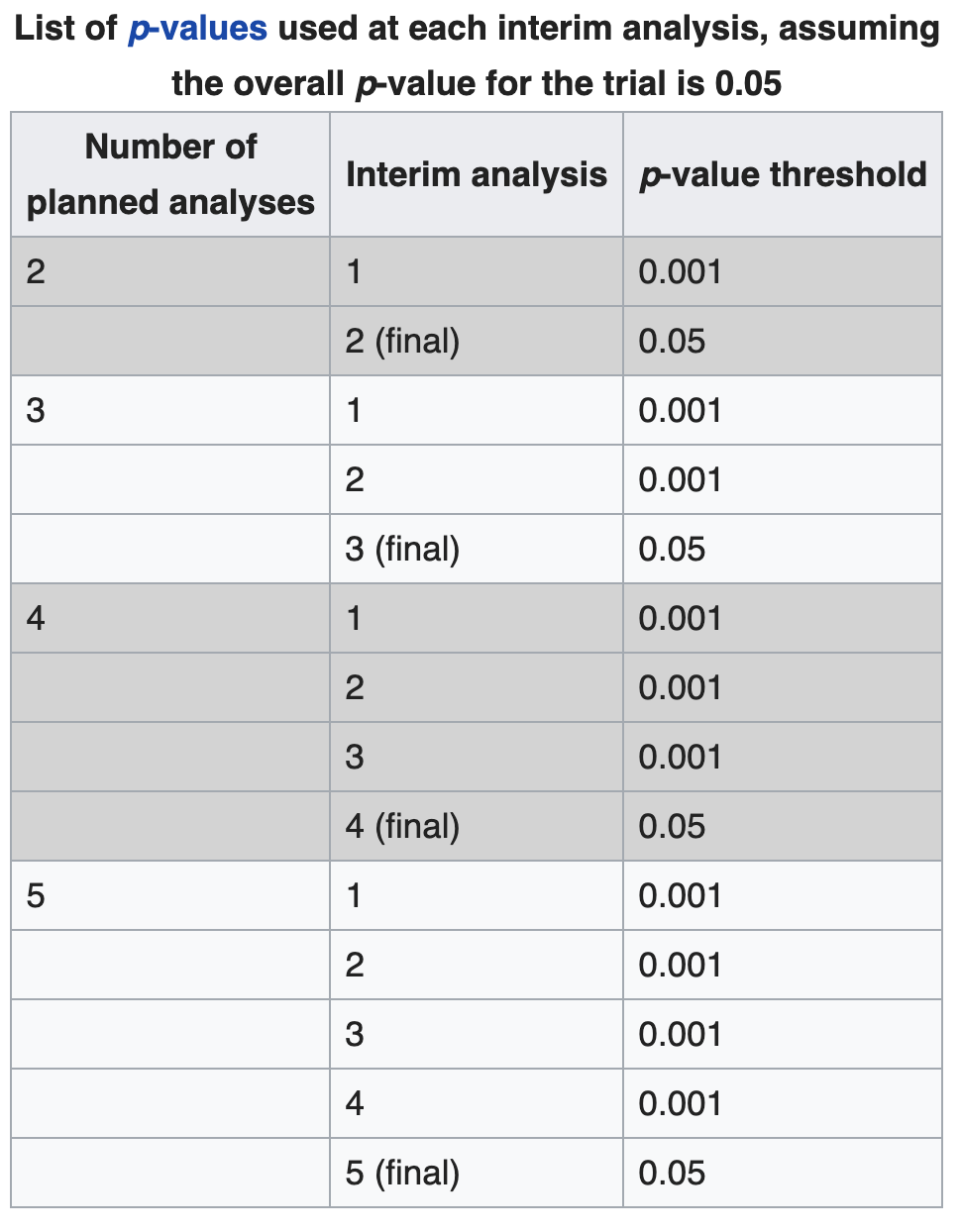
What this is essentially saying is: if you peek early and the null hypothesis is without a reasonable doubt wrong, ie. the treatment is without a reasonable doubt better than the control group already at lower $N$s, then stop, else keep going. More mathy, peak at some low $\alpha=\epsilon$, and your additional overall $\alpha$ will be some $\delta_\epsilon$ that is also low.
Ns = [1000] * 3
alphas = [0.001, 0.001, 0.05]

p = early_stopping_simulation(funnels, T, Ns, alphas)
print('False positive ratio: %.3f' % p)
Prints something like:
False positive ratio: 0.049
Obviously, there are countless protocols like this we can construct.
A final option is to not do this, never to stop the experiment until the original sample size of $N$ is reached. This is what I recommend to do. Note that peeking itself is not a problem, as long as we don’t stop the experiment. Some A/B testing tools go the extra mile and don’t show (blur out) the result before the agreed-upon sample size is reached.
What is the actual formula for the final $\alpha$, if we follow a protocol of testing at $\alpha_i$ at $N_i$ with early stopping? I’m not going to derive it here, we can just run the simulation above and see what it is. In the real-world, we don’t follow exact protocols like this anyway (peek at exact $N$ steps). In my opinion, it’s enough to be aware of this issue, and control our behaviour. I recommend to not early stop, or follow the conservative Haybittle–Peto boundary.
What’s the big deal?
Why do we even use A/B testing? Why don't we just eyeball the difference? After all, in a typical SaaS A/B testing setting, lives are not at stake, unlike in clinical trials.
We use formal A/B testing so we don’t fool ourselves. Usually the person or team performing the test has some attachment to the test, because it’s their idea, their code, they invested time into running the experiment, their bonus depends on their impact. We’re biased. By agreeing with ourselves or the team that we will follow a certain protocol to evaluate the experiment (sample size $N$, metric, $\alpha$), we’re eliminating or at least controlling our own bias.
But, we have to be mindful that A/B testing shouldn’t hold us back. In the post A/B tests: Moving Fast vs Being Sure I’ve argued that in startup settings it may make sense to run at higher $\alpha$ (and collect less samples per experiment), accept more false positives, because it will allow us to perform more experiments per year, which ultimately may be worth it.
Another thing to keep in mind that early stopping affects $\alpha$, the false positive rate. But false positives only matter for experiments that are not working, ie. when there is no lift from A to B. In the extreme case of all our experiments working, early stopping is actually good, because we will spend less time deciding, and we're "erring" in the right direction. But this is a extreme case, if all our experiments always work out, there’s no need to A/B test anyway.
We can do a back-of-the-envelope calculation to see what happens if we follow an early stopping protocol and (accidentally, or knowingly) run at $\alpha=0.10$ insteaf of $\alpha=0.05$. Let’s suppose that 1 in 4 ($\gamma=0.25$) experiment actually works, and we’re running at $1-\beta = 0.8$ power, ie. when an experiment works, we catch it 80% of the time. If we run 100 experiments a year:
- 25 will work, and we will catch 20 of these, 5 good ones will be misclassified as not working
- 75 will not work, if we run at:
- $\alpha=0.05$, then 3.75 bad ones will be misclassified as working
- $\alpha=0.10$, then 7.50 bad ones will be misclassified as working
The misclassification rate due to a $\Delta \alpha$ is $(1 - \gamma) \Delta \alpha$.
Conclusion
Increased false positive rate due to early stopping is beautiful nuance of statistical testing. It is equivalent to running at an overall higher $\alpha$. Data scientists need to be aware of this phenomenon so they can control it and keep their organizations honest about their experimental results.