Modern Portfolio Theory III: The Efficient Frontier in log volatility—return space
Marton Trencseni - Mon 30 December 2024 - Finance
Introduction
In the previous two articles, we explored the coverage of random portfolios in log volatility—return space, both with and without a risk-free asset:
- Modern Portfolio Theory I: Random portfolio coverage in log volatility—return space
- Modern Portfolio Theory II: Random portfolio coverage in log volatility—return space with a risk free asset
Note that the previous posts were using 2023 data, here we switch to 2024.
Modern Portfolio Theory (MPT), pioneered by Harry Markowitz in the 1950s, approaches portfolio construction by focusing on the trade-off between risk and return. At its core, MPT advocates for diversification — spreading investments across various assets to optimize the balance between expected return and risk. Central to this theory are two pivotal concepts:
-
Efficient Frontier: This is a graphical representation that showcases the set of optimal portfolios offering the highest expected return for a given level of risk (measured by volatility) or, conversely, the lowest risk for a desired level of return. Portfolios lying on the Efficient Frontier are deemed "efficient" because they maximize returns without incurring unnecessary risk.
-
Capital Market Line (CML): When a risk-free asset is introduced into the investment landscape, the CML emerges as a crucial tool. It represents the risk-return combinations achievable by combining the risk-free asset with portfolios on the Efficient Frontier. The CML not only illustrates the optimal trade-off between risk and return but also serves as a benchmark for evaluating the performance of investment portfolios.
We will now take the next step, and calculate the Efficient Frontier and Capital Market Line of Markowitz's theory in our framework. The ipython notebook is on Github.
Efficient frontier
At the heart of calculating the Efficient Frontier lies the ability to identify the optimal portfolio that offers the lowest possible risk (variance) for a given level of expected return. This optimization task is handled by the min_variance_portfolio() function in our Python code:
def min_variance_portfolio(means, cov_matrix, target_return):
    n = len(means)
    w0 = np.ones(n) / n # initial guess: equal weights
    constraints = [
        {'type': 'eq', 'fun': lambda w: np.sum(w) - 1},            # sum of weights = 1
        {'type': 'eq', 'fun': lambda w: means @ w - target_return} # target return: mu w
    ]
    bounds = [(0, 1)] * n # no short selling: weights >= 0
    # solve the optimization problem
    result = minimize(portfolio_variance, w0, args=(cov_matrix,),
                      constraints=constraints, bounds=bounds,
                      options={'ftol': 1e-9, 'maxiter': 1000})
    return result.x if result.success else None
The min_variance_portfolio() function is invoked iteratively across a range of target returns to map out the Efficient Frontier:
df_logr = np.log(df_nasdaq_100['Adj Close']).diff()[1:]
df_r = np.exp(df_logr)

means = df_r.mean()
cov_matrix = df_r.cov()

efficient_frontier = []
for tr in np.linspace(means.min(), means.max(), 100):
    portfolio = min_variance_portfolio(means, cov_matrix, tr)
    if portfolio is None:
        print(f'CSP failed for target return = {tr}')
        continue
    efficient_frontier.append((tr, portfolio))
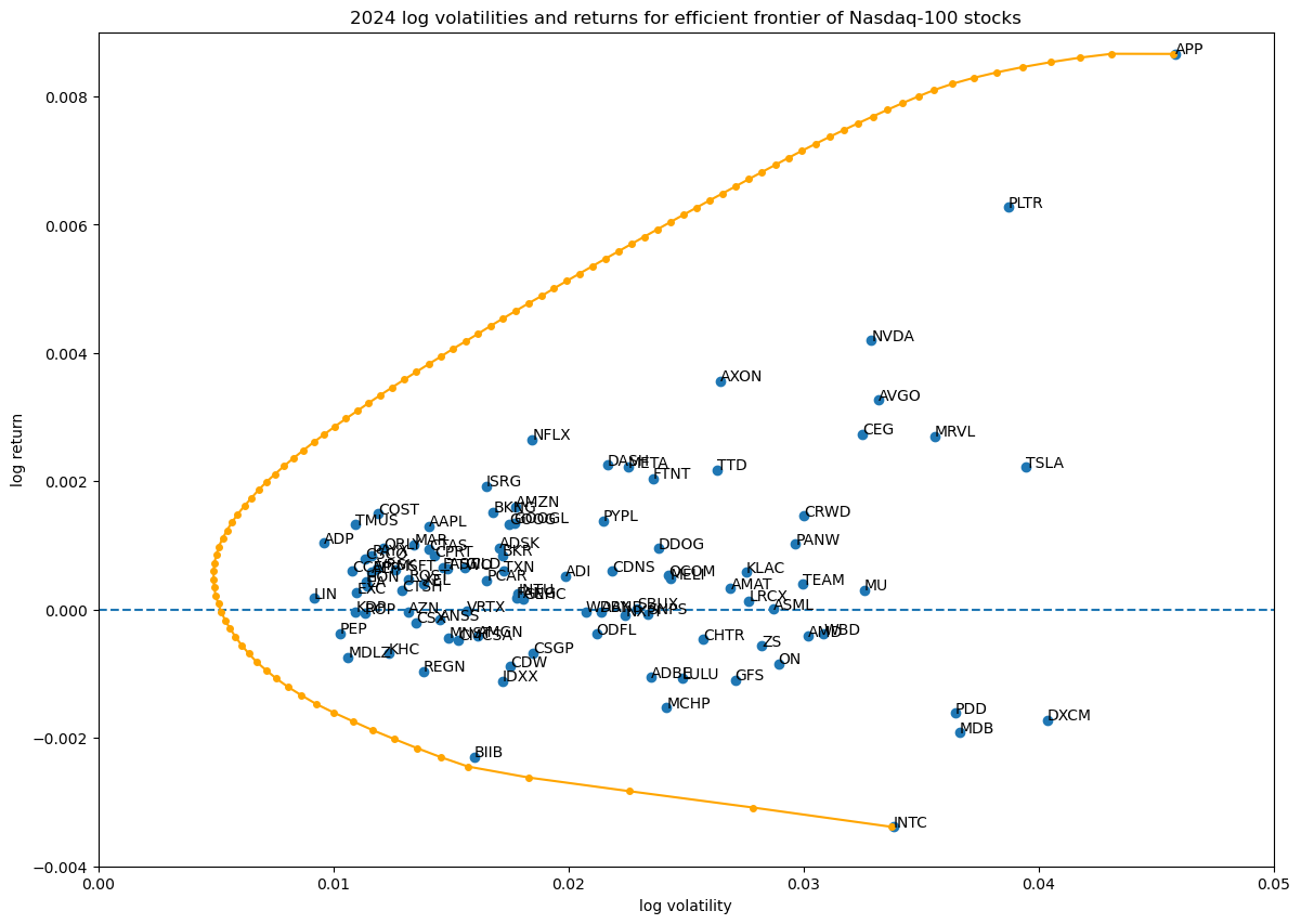
For each target return value, the function identifies the portfolio composition that achieves this return with the least possible risk. By aggregating these optimal portfolios, we form the Efficient Frontier—a curve that delineates the best trade-offs between risk and return available to an investor.
Efficient frontier without risk-free asset
Running the above code, we can see the shape of the Efficient Frontier:

Efficient frontier with risk-free asset
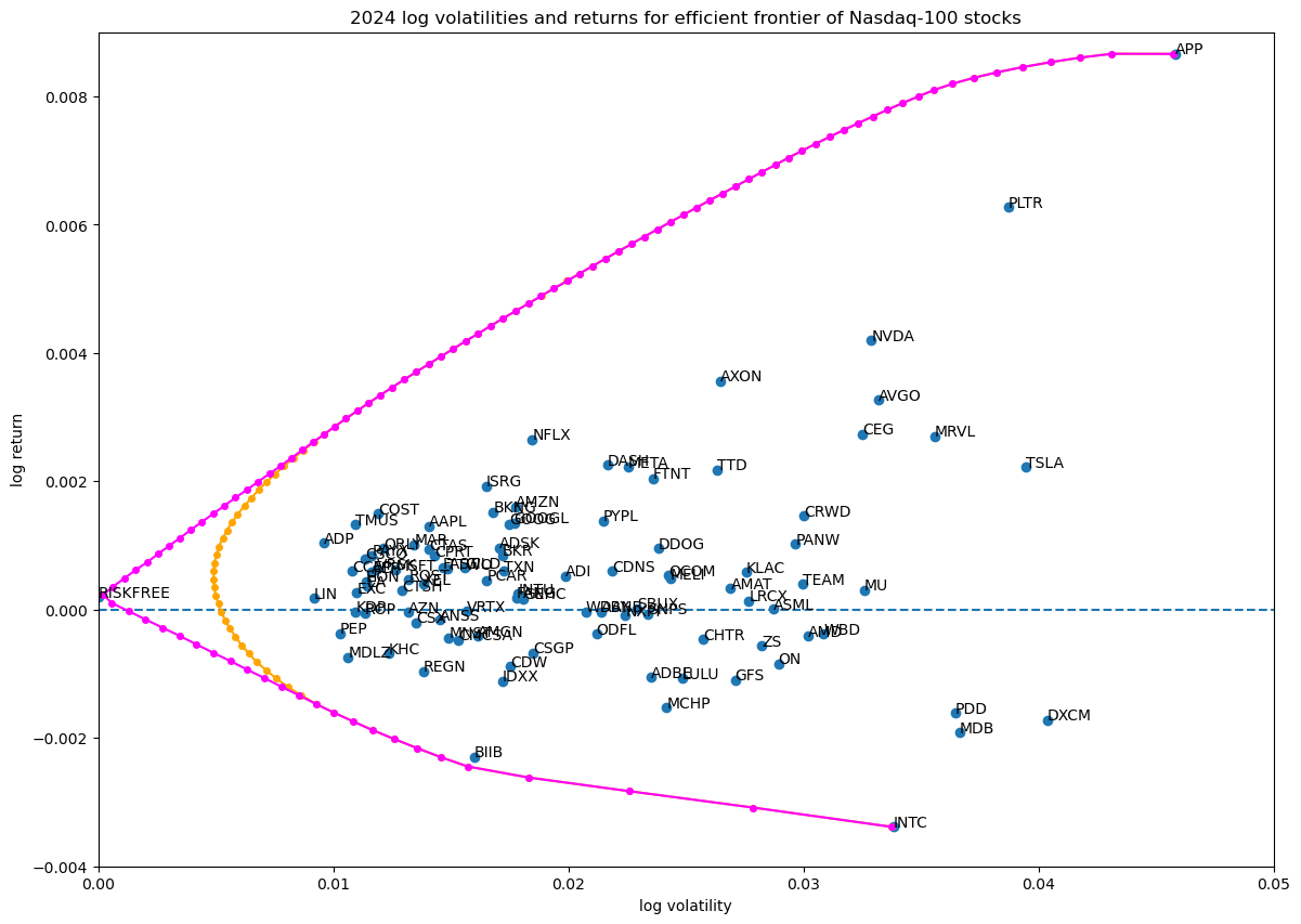
We can extend the efficient frontier with the Capital Market Line by injecting the risk-free asset into the portfolio and running the exact same code:
df_logr = np.log(df_nasdaq_100['Adj Close']).diff()[1:]
# inject the risk-free asset
risk_free_annual_return = 1.05
risk_free_daily_log_return = np.log(risk_free_annual_return**(1/len(df_logr)))
df_logr.insert(len(df_logr.columns), 'RISKFREE', [risk_free_daily_log_return] * len(df_logr))
df_r = np.exp(df_logr)
...
The orange line is the original efficient frontier, without the risk-free asset. The purple line is the efficient frontier with the risk-free asset, which now incorporates the Capital Market Line, the straight segment connecting the risk-free asset to the original hyperbola.

Conclusion
In the next post, I will combine random portfolios with the Efficient Frontier and also show the Sharpe ratio.