Probabilistic spin glass - Part IV

Introduction

In the previous articles (Part I, Part II, Part III) I looked at various properties of probabilistic spin glasses by simulating ensembles of many samples and computing various statistics, while in the case of entropy I computed probabilities directly. Then I let grids evolve over "time" by changing spins one by one.

In this final article I will run simulations to understand the scaling behaviour for large spin glasses. The ipython notebook is up on Github.

Scaling behaviour

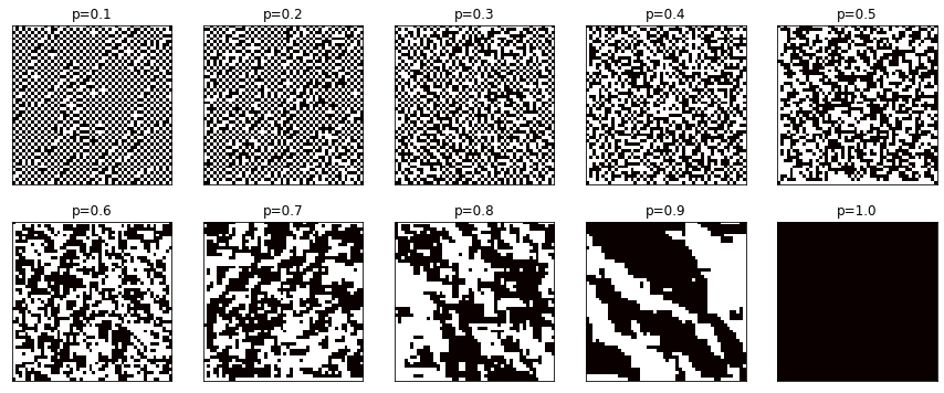
Let's see what different size spin glasses look like at different $P(s=1|n=1)=p$ values. Here are $50 \times 50$ grids:

Here are $500 \times 500$ grids, so each of these grids is $10 \times 10 = 100$ times larger than the previous ones:

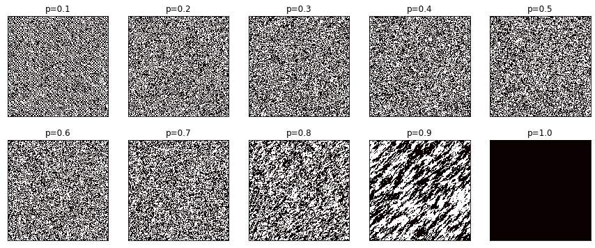
These look quite different! In the $500 \times 500$ case, the $p=0.7$ and even the $p=0.8$ look like random noise, whereas for the smaller grid, we see the deviation from random noise much earlier.

This behaviour is quite interesting. Actually, each $50 \times 50$ part of the larger $500 \times 500$ grid looks about the same as the corresponding smaller grid, if we were to zoom in. But with a larger grid, there are more chances for the spins to mis-align, so even if there is a block of ↑ spins, eventually there will come a block of ↓ spins. For a smaller grid, this also happens, but there is less space for it to happen, so the grid is more likely to show a pattern. And for a large enough grid, in the zoomed out view, these will look like random specks of noise.

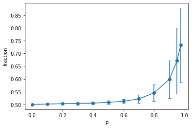
We can quantify the above by drawaing the majority fraction of the spins. This is just the fraction of the spins that all ↑ or ↓, whichever is more. In the previous article, we already looked at this, with the standard deviation of this fraction:

Let's draw the same curve, but for different sized grids. Let's look at the average and standard deviation seperately using our usual Monte Carlo measurement method:

# Monte Carlo measurement
p0, num_samples = 0.5, 100
measurements = []
for p in [0.1, 0.2, 0.3, 0.4, 0.5, 0.6, 0.7, 0.8, 0.9, 0.95, 0.975]:
    for N in [50, 100, 200, 500]:
        rs = [fraction(create_grid_symmetric(rows=N, cols=N, p0=p0, p=p)) for _ in range(num_samples)]
        measurements.append((N, p, np.mean(rs), np.std(rs)))
# plot
fig, axs = plt.subplots(1, 2, figsize=(15, 6))
Ns = sorted(list(set([x[0] for x in measurements])))
for N in Ns:
    pts = sorted([(x[1], x[2], x[3]) for x in measurements if x[0] == N])
    axs[0].plot([x[0] for x in pts], [x[1] for x in pts], marker='o')
    axs[0].set_xlabel('p')
    axs[0].set_ylabel('majority fraction')
    axs[1].plot([x[0] for x in pts], [x[2] for x in pts], marker='o')
    axs[1].set_xlabel('p')
    axs[1].set_ylabel('stdev. of majority fraction')
    axs[1].legend([f'{N}x{N}' for N in Ns])

Yields:

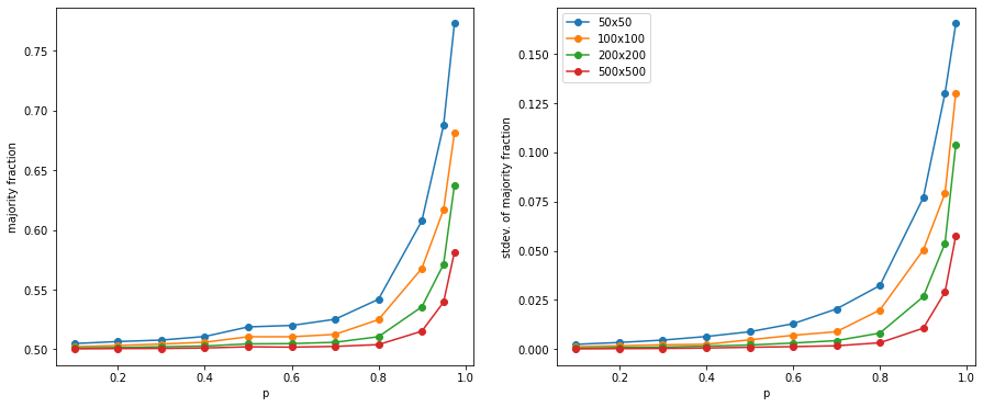
This confirms the above. As the grid size gets larger, the (mean) majority fraction gets pushed down, as does its standard deviation. So in the limiting case, for an infinitely large grid, the majority fraction curve would get pushed down to 0.5, and then jump to 1 at $p=1$ (if $p=1$, all the spins have to align).

Conclusion

In retrospect, the above scaling behaviour makes sense, but it was not expected. I thought it follows the same fraction-curve at all grid sizes.