The Unreasonable Effectiveness of Monte Carlo Simulations in A/B Testing

Introduction

In his influential essay, The Unreasonable Effectiveness of Mathematics in the Natural Sciences (pdf), the Hungarian physicist Eugene Wigner marveled at the uncanny ability of abstract mathematics to describe and predict the physical world with remarkable precision. Wigner pondered how mathematical concepts, developed independently of empirical observations, could so effectively model the complexities of nature. This profound connection between mathematics and the natural sciences has been a cornerstone in advancing our understanding of the universe.

Building upon this theme, Peter Norvig's article, The Unreasonable Effectiveness of Data (pdf), emphasizes how vast amounts of data available today empower us to solve problems that were previously inaccessible. Norvig argues that with sufficient data, simple models can outperform more sophisticated ones, highlighting the pivotal role of data over complex algorithms. This shift toward leveraging abundant information mirrors a broader trend in scientific computation.

In a similar vein, Monte Carlo simulations are an effective tool across various scientific and engineering disciplines. Originating from statistical physics and named after the famed casino city due to their reliance on randomness, Monte Carlo methods harness random sampling to approximate solutions to problems. However, their utility extends beyond tackling analytically intractable challenges. Monte Carlo simulations also allow us to directly simulate systems with known solutions, providing intuitive insights into why those solutions are what they are. By experimenting computationally, we can observe how changes in parameters affect outcomes, thereby deepening our understanding of the underlying processes—a practice that could be referred to as the computational experimentalist's calculus.

By running computational experiments that rely on random sampling, Monte Carlo simulations enable us to explore complex systems interactively. They serve as a bridge between theoretical models and practical applications, allowing us to validate analytical solutions, investigate their sensitivities, and intuitively grasp their implications. This approach is especially valuable in an era where computational resources are abundant and hands-on experimentation can complement traditional analytical methods.

Historical context

The origins of Monte Carlo methods date back to the 1940s during the development of nuclear weapons in the Manhattan Project. Physicist Stanislaw Ulam conceived the idea while recovering from an illness and playing solitaire games. He pondered whether the chance of winning could be calculated by simulating numerous random deals rather than attempting a daunting combinatorial analysis.

Collaborating with Hungarian physicist John von Neumann and Nicholas Metropolis, Ulam applied this concept to model neutron diffusion in fissile materials — a problem too complex for analytical solutions due to the multitude of interacting particles. The term "Monte Carlo" was coined by Metropolis, referencing the famed casino city in Monaco, alluding to the randomness and chance inherent in the methods.

Since then, Monte Carlo methods have been adopted across a multitude of disciplines:

• Physics: Modeling particle interactions, quantum mechanics, and statistical physics phenomena.
• Finance: Pricing complex derivatives, risk assessment, and portfolio optimization.
• Engineering: Solving integral equations, optimization problems, and reliability analysis.
• Computer Graphics: Rendering images using ray tracing and global illumination techniques.
• Statistics: Performing Bayesian inference and simulating sampling distributions.

The advent of modern computers significantly boosted the practicality of Monte Carlo simulations, enabling the handling of computations involving millions or billions of random samples.

Monte Carlo methods are particularly effective for several reasons:

• Simplicity of Implementation: Implementing a Monte Carlo simulation often requires fewer lines of code compared to analytical or deterministic numerical methods. By focusing on random sampling and aggregation, they reduce the need for intricate mathematical derivations.
• Insight Through Experimentation: By directly simulating the system, we gain intuitive understanding of how different factors influence outcomes. This experimental approach allows us to tweak parameters, observe effects, and develop hypotheses—much like conducting physical experiments in a virtual environment.
• Parallelization and Computational Efficiency: The independent nature of random sampling makes Monte Carlo simulations well-suited for parallel computing. Modern multi-core processors, GPUs and distributed computing systems can perform numerous simulations simultaneously, drastically reducing computation time.

The Python program below illustrates the simplicity of Monte Carlo by estimating the mathematical constant $ \pi $ in essentially one line of code:

from random import random
from math import pi
np.random.seed(7989) # reproducibility

N = 100_000_000
pi_estimate = 4 * sum([1 for _ in range(N) if random()**2 + random()**2 < 1]) / N

print('Actual:   %.3f' % pi)
print('Estimate: %.3f' % pi_estimate)

Output:

Actual:   3.142
Estimate: 3.142

By using randomness, Monte Carlo simulations offer a powerful means to approximate solutions where traditional methods are infeasible or inefficient. They democratize problem-solving by providing accessible tools that require less specialized mathematical background, allowing practitioners to focus on experimentation and exploration.

In essence, Monte Carlo methods embody the idea that sometimes, the most effective way to understand a complex system is not through exhaustive analytical solutions but through the aggregation of many simple, random trials. This approach aligns with the increasing availability of computational resources, making it an indispensable asset in modern science and engineering.

See the Bytepawn article Estimating mathematical constants with Monte Carlo simulations for more examples of calculating mathematical constants using Monte Carlo methods.

The rise of A/B testing

Randomized Controlled Trials (RCTs) have long been the gold standard in experimental research, particularly in medicine and social sciences. By randomly assigning subjects to control and treatment groups, RCTs aim to eliminate bias and establish causal relationships between interventions and outcomes.

With the advent of the internet and digital platforms, the principles of RCTs were adapted into what we now call A/B testing. This method allows businesses to compare two versions of a webpage, app feature, or any user interface element to determine which performs better according to predefined metrics. A/B testing empowers companies to make data-driven decisions, optimize user engagement, enhance conversion rates, and thus maximize revenues and profits.

However, the simplicity of setting up A/B tests belies the complexity of interpreting their results correctly. Issues such as p-hacking, misunderstanding statistical significance, and improper test design can lead to erroneous conclusions. This is where Monte Carlo simulations become invaluable, providing clarity and insight into the statistical mechanisms underlying A/B testing. The experimenter can simply implement their experimental framework and assumptions as a simple Python program and run Monte Carlo simulations to explore its statistical properties.

The remainder of the article will discuss examples of using Monte Carlo simulations to understand aspects of A/B testing.

See the all Bytepawn articles tagged with ab-testing for more in-depth articles on A/B testing.

False positive rate and Statistical power

Understanding false positives and statistical power is crucial in A/B testing, yet these concepts can sometimes feel abstract. Monte Carlo simulations offer a powerful way to visualize and comprehend these statistical phenomena by simulating thousands of experiments and observing their outcomes.

Simulating False Positives (Type I Errors) A false positive, or Type I error, occurs when we incorrectly conclude that there is a significant difference between two groups when, in reality, there isn't one. In the context of A/B testing, this means detecting an effect that doesn't exist.

To illustrate this, let's simulate an A/A test where both groups A and B have the same true conversion rate of 10%. We'll perform $ S = 10\,000 $ simulations, each time with a large sample size of $ N = 1\,000\,000 $ users per group. The significance level $ \alpha $ is set at 0.05.

import numpy as np
import scipy.stats as stats
np.random.seed(7989)  # reproducibility

# Parameters
conversion_rate = 0.1    # true conversion rate for both groups
sample_size = 1_000_000  # number of samples in each group
num_simulations = 10_000 # number of simulations
alpha = 0.05             # significance level

def compute_p_value_one_tailed(conversions_A, conversions_B, N):
    pooled_cr = (conversions_A + conversions_B) / (2 * N)
    s_error = np.sqrt(2 * pooled_cr * (1 - pooled_cr) / N)
    z_score = (conversions_B - conversions_A) / (N * s_error)
    p_value = 1 - stats.norm.cdf(abs(z_score))
    return p_value

# Function to perform one A/B test simulation
def simulate_ab_test(conversion_rate, N, lift=0):
    # Simulate conversions for group A and B under null hypothesis
    conversions_A = np.random.binomial(N, conversion_rate)
    conversions_B = np.random.binomial(N, conversion_rate * (1 + lift))
    if conversions_B > conversions_A:
        return compute_p_value_one_tailed(conversions_A, conversions_B, sample_size)
    else:
        return 1.0

Let's look at the scenario of an A/A test, when there is no difference between the two variants, the lift is 0%. Any statistically significant difference detected is a false positive.

# simulate an A/A test where A and B are the same
lift = 0.0
p_values = [simulate_ab_test(conversion_rate, sample_size, lift) for _ in range(num_simulations)]
# calculate False Positive Rate (FPR) a.k.a. Type I Error rate
# this is the proportion of cases when the p-value was below alpha
# ie. we would falsely conclude that B is better than A
type_I_errors = np.sum(np.array(p_values) < alpha) / num_simulations
print(f"Type I Error rate: {type_I_errors:.3f}")

Output:

Type I Error rate: 0.051

Interpretation:

• Out of $ 10\,000 $ simulations, approximately 5% resulted in p-values less than 0.05.
• This aligns with our significance level $ \alpha = 0.05 $, confirming that the probability of a Type I Error is controlled by $ \alpha $.
• Even when there is no true difference, we expect to see some false positives purely due to chance.

Next, we simulate an A/B test where the treatment group has a 1% relative improvement in the conversion rate.

# simulate an A/B test where B is relative 1% better than A
lift = 0.01
p_values = [simulate_ab_test(conversion_rate, sample_size, lift) for _ in range(num_simulations)]
# calculate Statistical Power
# this is the proportion of cases when the p-value was below alpha
# ie. we would catch that B is better than A
statistical_power = np.sum(np.array(p_values) < alpha) / num_simulations
print(f"Statistical power: {statistical_power:.3f}")

Output:

Statistical power: 0.763

Interpretation:

• The statistical power is about 76.3%, indicating a 3 in 4 chance of detecting a true effect of 1% lift.
• The risk of a Type II Error (false negative) is 23.7% in this scenario.

These simulations highlight the effectiveness of Monte Carlo methods:

• By simulating thousands of experiments, we observe how random chance can lead to false positives and how true effects are detected.
• The observed Type I Error rate matches the significance level.
• Statistical power was not explicitly specified in the parameters, it is a function or result of the chosen values.
• The experimenter can then vary the sample size to see how to achieve a potentially desired higher statistical power at a given lift.

Monte Carlo simulations make abstract statistical concepts tangible, helping us grasp the real-world implications of our testing strategies.

Early stopping

Early stopping in A/B testing is a critical consideration that can significantly impact the validity of experimental results. In a standard experimental protocol, we begin by defining the evaluation metric—selecting a key performance indicator such as conversion rate, time spent, or daily active users. Next, we determine the sample size $ N $ required to achieve sufficient statistical power, choose the appropriate statistical test based on the data characteristics (such as a t-test or chi-squared test), and set the significance level $ \alpha $, which establishes the acceptable false positive rate, commonly at 0.05. We then collect data by running the experiment until the predetermined sample size is reached and analyze the results by performing the statistical test and interpreting the p-value to accept or reject the null hypothesis.

However, in practice, experimenters often face the temptation of early stopping—the act of peeking at the data before the experiment reaches the planned sample size and making decisions based on interim results. While this may seem like a way to expedite decision-making, early stopping can significantly inflate the false positive rate, leading to incorrect conclusions.

Early stopping disrupts the statistical integrity of the experiment. Each time we perform an interim analysis and test for significance, there's a chance of observing a false positive purely by random chance. If we repeatedly check the data and stop the experiment once we achieve statistical significance, we inadvertently increase the overall probability of committing a Type I Error (false positive). For instance, suppose we plan to collect $ N = 3\,000 $ samples but decide to peek at the results every $ 1\,000 $ samples. At each interim analysis, we perform a statistical test at the significance level $ \alpha = 0.05 $. The cumulative effect of conducting multiple tests increases the overall false positive rate beyond the nominal 5%. In fact, simulations show that with three such analyses, the false positive rate can nearly double.

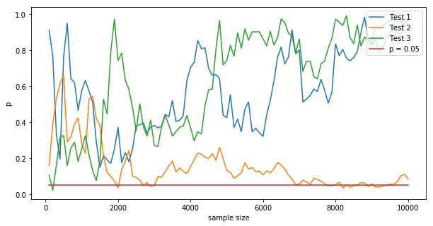
The intuition behind this increase lies in the nature of p-values and random variability. Under the null hypothesis (no real difference between variants A and B), p-values are uniformly distributed between 0 and 1. This means that at any given time, there's always a probability $ \alpha $ of observing a p-value less than the significance threshold $ \alpha $ purely by chance. When we perform multiple interim analyses, each one provides an additional opportunity to cross the significance threshold due to random fluctuations in the data. The more we peek, the higher the chance that we'll observe a statistically significant result when there is no true effect. This is shown in the figure below, illustrating the p-values for three A/A test simulations runs, evaluated every 100 samples, 100 times for a total of $ N=10\,000$ samples.

Monte Carlo simulations offer a powerful means to visualize and quantify the effects of early stopping. By simulating numerous experiments under the null hypothesis and mimicking the early stopping protocol, we can observe how the false positive rate escalates with each additional interim analysis. These simulations demonstrate that the overall false positive rate increases substantially compared to a single analysis at the end of the experiment, highlighting the risks associated with early stopping.

To mitigate the increased false positive rate while allowing for interim analyses, statisticians have developed methods to control the overall Type I error rate. One such approach is alpha spending, which distributes the total allowable Type I error ($ \alpha $) across multiple analyses. For example, Pocock's boundary adjusts the significance level to be more stringent at each interim analysis. If we plan three analyses and want to maintain an overall $ \alpha = 0.05 $, we might set the significance level at each analysis to $ \alpha' = 0.0221 $. This adjustment ensures that the cumulative probability of a Type I error across all analyses remains at the desired level.

Another approach is the Haybittle–Peto boundary, which sets a very stringent significance level (e.g., $ \alpha = 0.001 $) for interim analyses and retains the standard $ \alpha = 0.05 $ for the final analysis. This method is simple and conservative, effectively controlling the overall false positive rate without complex calculations. Monte Carlo simulations can validate these adjusted thresholds by demonstrating that the overall false positive rate remains at the intended level when these methods are applied.

It's important to consider the context in which the experiment is conducted. In some cases, accepting a higher false positive rate might be tolerable if the cost of a false positive is low and the benefit of early detection is high. This trade-off should be made consciously and transparently.

Monte Carlo simulations serve as a valuable tool for understanding and communicating the impact of early stopping. By modeling various scenarios and observing the outcomes, experimenters can visualize the risk of increased false positives and evaluate the effectiveness of different alpha spending methods. These simulations bridge the gap between abstract statistical theory and practical application, making it easier to grasp the consequences of methodological choices.

In essence, early stopping in A/B testing poses a significant risk to the validity of experimental results by inflating the false positive rate. While the allure of quick wins is strong, especially in fast-paced business environments, maintaining statistical rigor is essential for making reliable data-driven decisions. Being mindful of the statistical underpinnings of A/B testing and leveraging tools like Monte Carlo simulations enhances the effectiveness of experiments and contributes to more robust and impactful decision-making.

See the Bytepawn article Early stopping in A/B testing for a more in-depth explanation with code samples and figures.

Variance Reduction Techniques

In A/B testing, accurately detecting differences between two groups hinges on minimizing variance in the measurements. When we compare the means of a metric—such as user spend or conversion rates—across control and treatment groups, the Central Limit Theorem assures us that the sampling distribution of the mean approximates a normal distribution. Consequently, the difference between the two group means (often referred to as the lift) also follows a normal distribution, with its variance being the sum of the variances of each group. Reducing this variance is crucial for increasing the precision and reliability of our experimental results. See the Bytepawn article A/B testing and the Central Limit Theorem for a more in-depth exploration of the CLT with Monte Carlo methods.

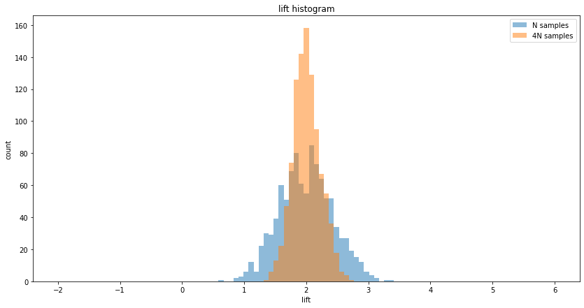
The most straightforward way to reduce variance is by increasing the sample size. According to statistical principles, the variance of the sample mean decreases proportionally with the increase in sample size. Specifically, quadrupling the number of observations halves the standard error. While this method is effective, practical limitations often arise, as illustrated in the figure above drawn by running Monte Carlo simulations. Collecting more data may not be feasible due to time constraints, resource limitations, or the finite availability of participants. Additionally, extending the duration of an experiment doesn't always yield a proportional increase in unique users, as returning visitors may inflate sample counts without providing new information.

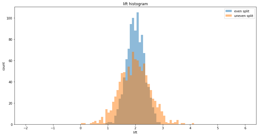
Allocating participants equally between the control and treatment groups minimizes variance in the estimated effect size. When the total sample size is fixed, a 50%-50% split ensures the lowest possible variance for the difference between group means. Deviations from an even split increase variance because the variance of each group's mean is inversely proportional to its sample size. An uneven allocation, such as 90%-10%, results in a higher combined variance compared to an even split, as illustrated in the figure above. Therefore, when feasible, it's advisable to distribute participants equally to enhance the sensitivity of the experiment.

Another approach to variance reduction involves refining the metric itself to make it less variable. This can be achieved through:

• Winsorizing or trimming outliers: Extreme values can disproportionately inflate variance and obscure true effects. By capping or removing outliers beyond a certain threshold, we focus the analysis on the central tendency of the data. For instance, in measuring spend per user, extraordinarily high purchases might be due to anomalous behavior or errors and can be capped to reduce their impact.

• Using medians instead of means: The median is less sensitive to extreme values and can provide a more robust measure when the data distribution is skewed. However, statistical tests for medians may have different properties and may require non-parametric methods.

• Focusing on relevant subpopulations: By segmenting users into more homogeneous groups based on characteristics like engagement level or purchase history, we can reduce within-group variance. Analyzing these subpopulations separately can yield more precise estimates.

• Splitting metrics: Decomposing a complex metric into its components can reduce variance. For example, overall spend per user can be split into the conversion rate (the proportion of users who make a purchase) and the average spend among purchasers. Each component typically has lower variance than the combined metric, and analyzing them separately can provide clearer insights.

Stratified sampling involves dividing the overall sample into distinct subgroups or strata based on specific characteristics, such as age, gender, or previous behavior, and ensuring that these strata are equally represented in both control and treatment groups. This method reduces variance by controlling for variability within these subgroups and preventing imbalance that could confound the results. By ensuring that each subgroup contributes proportionally to both groups, we eliminate potential sources of variance unrelated to the treatment effect. Stratification is particularly effective when the outcome metric varies significantly across these subgroups.

Incorporating covariates—additional variables that are correlated with the outcome metric—can significantly reduce variance. CUPED (Controlled Experiment Using Pre-Experiment Data) is a technique that adjusts for variance using covariates measured before the experiment begins. If historical data on the outcome metric is available, and there is a strong correlation between past and current behavior, this information can be used to adjust the post-treatment measurements. See all Bytepawn articles tagged with cuped for an in-depth exploration of CUPED using Monte Carlo methods.

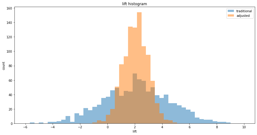
CUPED works by computing an adjusted metric that accounts for the covariance between the pre-experiment and post-experiment data. This adjustment effectively removes the portion of variance explained by the covariate, leading to a more precise estimate of the treatment effect, as illustrated in the figure above. For example, if users who spent more before the experiment tend to spend more during the experiment, using their prior spend as a covariate can control for this variability.

See the Bytepawn article Five ways to reduce variance in A/B testing for more information and code on variance reduction techniques, explored using Monte Carlo simulations.

Frequentist and Bayesian A/B testing

In the practice of A/B testing, two predominant statistical frameworks guide our analysis: frequentist statistics and Bayesian inference. Both aim to determine whether a new variant (B) performs differently from a control (A), but they approach the problem from different philosophical standpoints and methodologies.

The frequentist approach (which we have used up until now) revolves around the formulation of hypotheses. We set up a null hypothesis $ H_0 $, which typically states that there is no difference between the conversion rates of A and B — that any observed difference is due to random chance. The alternative hypothesis $ H_1 $ (sometimes called the action hypothesis) posits that there is a significant difference, with B performing better than A. After running the experiment, we calculate a p-value $ p_f $ ($f$ for frequentist), which represents the probability of observing data at least as extreme as the actual results, assuming the null hypothesis is true. If this p-value is lower than a predetermined significance level (commonly $ \alpha = 0.05 $ or $ 0.01 $), we reject the null hypothesis in favor of the alternative, concluding that the treatment has a statistically significant effect.

On the other hand, the Bayesian approach flips this perspective. Instead of focusing on the probability of the data given the null hypothesis, it computes the probability that the alternative hypothesis is true given the observed data. This involves using Bayes' theorem to update our prior beliefs about the parameters of interest based on the experimental outcomes, resulting in a posterior probability $ p_b $ ($b$ for bayesian). In A/B testing, we model the conversion probabilities of A and B using probability distributions, often choosing the Beta distribution due to its suitability for modeling probabilities between 0 and 1.

The Beta distribution is parameterized by two parameters, $ \alpha $ and $ \beta $, corresponding to the number of successes (conversions) and failures (non-conversions), respectively. Given the observed data—say, $ C $ conversions out of $ N $ trials—we set $ \alpha = C $ and $ \beta = N - C $ for each variant. This allows us to express our uncertainty about the true conversion rate of each variant as a probability distribution. To determine the probability that B is better than A, we compute $ P(\mu_B > \mu_A) $, where $ \mu_A $ and $ \mu_B $ are the true conversion rates of A and B. This involves integrating the joint probability distribution over the region where $ \mu_B > \mu_A $. While sometimes a closed-form solution exists, we often use Monte Carlo integration by sampling from the Beta distributions of both A and B and estimating the proportion of times $ \mu_B > \mu_A $.

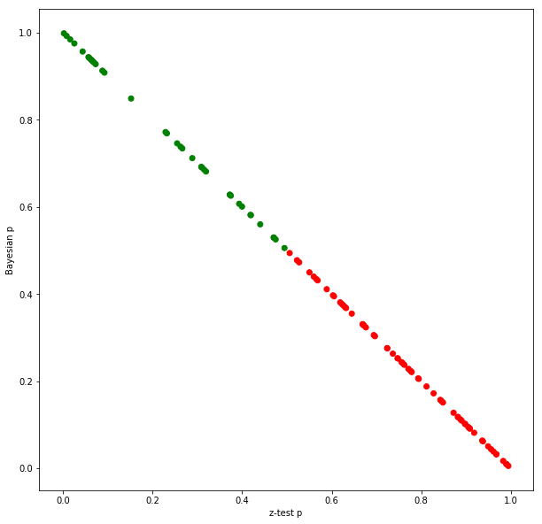
An intriguing observation emerges when comparing the frequentist p-value $ p_f $ and the Bayesian posterior probability $ p_b $. Under certain conditions—specifically, when using flat priors and with sufficiently large sample sizes—the relationship $ p_f + p_b \approx 1 $ holds, as illustrated in the figure above using Monte Carlo methods. This suggests that, in these scenarios, the frequentist and Bayesian methods provide complementary perspectives on the same data. However, this is an approximation and does not hold exactly, especially with small sample sizes or strong prior beliefs.

To delve deeper, consider that in frequentist inference, particularly when using the z-test, we rely on the Central Limit Theorem (CLT) to approximate the sampling distribution of the conversion rates as normal distributions. The difference in conversion rates between A and B is also normally distributed, centered on the observed difference, with a variance that depends on the individual variances of A and B. We then calculate the probability of observing a difference at least as extreme as the one observed under the assumption that the null hypothesis is true.

In Bayesian modeling, when we use Beta distributions with weak or non-informative priors, and when sample sizes are large enough for the Beta distributions to approximate normal distributions (thanks to the CLT), the posterior distributions of the conversion rates become similar to the frequentist normal approximations. This convergence explains why $ p_f + p_b \approx 1 $ holds under these conditions.

However, the choice of prior in Bayesian analysis can significantly impact the results. If we use a strong prior, such as $ \text{Beta}(\alpha_0, \beta_0) $ with large $ \alpha_0 $ and $ \beta_0 $, our prior beliefs may dominate the posterior distribution, requiring substantial new data to shift our confidence. This means that with strong priors, the approximation $ p_f + p_b \approx 1 $ may not hold, and the Bayesian probability $ p_b $ may remain relatively unchanged despite new data.

Monte Carlo simulations play a crucial role in bridging these concepts. By simulating a large number of experiments, we can visualize how the Bayesian posterior probability $ p_b $ and the frequentist p-value $ p_f $ behave under different conditions. For instance, with small sample sizes or extreme conversion rates (close to 0 or 1), the Beta distributions differ significantly from the normal approximations, and the relationship between $ p_f $ and $ p_b $ becomes less predictable.

Understanding these differences is essential for making informed decisions in A/B testing. The frequentist p-value does not give us the probability that the alternative hypothesis is true — it tells us how unusual our data is under the null hypothesis. Conversely, the Bayesian posterior probability $ p_b $ directly addresses the question of how likely it is that B is better than A, given our prior beliefs and the observed data.

See the Bytepawn article Bayesian A/B conversion tests for an in-depth explanation of the concepts above using Monte Carlo simulations.

Conclusion

Monte Carlo simulations offer a way to visualize and internalize the behavior of statistical metrics under various scenarios. They transform abstract mathematical notions into tangible experiences, allowing us to see the probabilities unfold through thousands of simulated experiments. This not only enhances our intuition but also equips us with the confidence to design better experiments and make more informed decisions based on data.

Yet, as Eugene Wigner astutely remarked, "It's nice to know that the computer understands the problem. But I would like to understand it too." This sentiment underscores the importance of not relying solely on computational power but also striving for a deep, conceptual grasp of the statistical principles at play. While computers can perform vast calculations and process immense datasets, it is our responsibility to interpret the results, question assumptions, and ensure that our conclusions are both valid and meaningful.

The unreasonable effectiveness of Monte Carlo simulations lies not just in their computational prowess but in their ability to enhance human understanding. They serve as a bridge between the complexity of statistical theory and the practical needs of experimenters seeking actionable insights. By using simulations to explore the nuances of A/B testing, we become better equipped to avoid common pitfalls, such as misinterpreting p-values or succumbing to the allure of early stopping without proper adjustments.

By integrating Monte Carlo simulations into our A/B testing toolkit, we enhance our ability to design robust experiments, interpret results accurately, and make decisions that are both statistically sound and practically relevant. This fusion of computational power and human understanding empowers us to navigate the complexities of modern data analysis with confidence and precision.