Probabilistic spin glass - Part V

Introduction

In the previous articles I looked at various properties of probabilistic spin glasses by simulating ensembles of many samples and computing various statistics, while in the case of entropy I computed probabilities directly. Then I let grids evolve dynamically over "time" by changing spins one by one. In the previous article I ran simulations to understand the ensemble scaling behaviour for large spin glasses:

• Part I
• Part II
• Part III
• Part IV

Now I will revisit the dynamic behaviour and see how the saturation behaviour scales with $p$ and $N$. The ipython notebook is on Github.

Saturation behaviour

Let's take a periodic $N \times N$ spin glass with $P(s=1|n=1)=p$ and let it evolve over time. One evolution step is taking a random spin, ignoring its current state, and based on the surrounding four states probabilistically setting a new state. Let's define a frame to be $N \times N$ such steps, so that on average each spin gets one chance to change per frame.

What I am interested here is the saturation behaviour of the spin glass. Saturation is when the majority of the spins align in one direction, whether that direction is ↑ or ↓. Since we're running probabilistic simulations, the ratio of aligned spins will not be exactly 1.0; we define a saturation threshold, above which we say that "essentially" all spins are aligned. For the smallest considered $10 \times 10$ spin glass let's use satuation_limit=0.90, for larger ones saturation_limit=0.95.

Let's take a $N \times N$ spin glass, and let it evolve for 1000 frames, using different $p$s. At each frame, let's plot the saturation, ie. the majority spin ratio. Let's repeat this for 100 different trajectories, and record the ratio of trajectories where the spin glass saturated (this will be shown in the plot titles like sat=0.8 meaning 80% of trajectories saturated ie. reached the saturation_limit of aligned spins). The code for this:

def get_saturation(N, p0, starting_ps, ps, num_frames,
                   n_jobs, num_trajectories_per_job, saturation_limit, draw_plots=True):
    if draw_plots: fig, axs = plt.subplots(1, len(ps), figsize=(20, 4))
    results = []
    for i, (starting_p, p) in enumerate(zip(starting_ps, ps)):
        trajectories = Parallel(n_jobs=n_jobs)(delayed(get_trajectories_periodic)
                                (rows=N, cols=N, p0=p0, starting_p=p, p=p,
                                 num_trajectories=num_trajectories_per_job,
                                 num_frames=num_frames, random_seed=i)
                                for i in range(n_jobs))
        trajectories = list(itertools.chain(*trajectories))
        saturation = np.mean([np.mean(t[-10:]) > saturation_limit for t in trajectories])
        results.append((N, p0, starting_p, p, saturation, trajectories))
        for trajectory in trajectories:
            if draw_plots: axs[i].plot(trajectory)
        if draw_plots: axs[i].set_ylim((0.49, 1.0))
        if draw_plots: axs[i].set_title(f'N={N}, start_p={starting_p:.3f}, p={p:.3f}, sat={saturation:.2f}')
    if draw_plots: plt.show()
    return results

Note the use of Parallel() to use all available cores for Monte Carlo simulation. I ran this with 20x parallelism for more sample size.

We can run this for different sized spin glasses. In each of the trajectories, let's start with a random noise starting_p=0.5 spin glass:

# fixed starting_p=0.5
p0, starting_p, num_frames, n_jobs, num_trajectories_per_job = 0.5, 0.5, 1000, 20, 5
ps = [0.50, 0.75, 0.90, 0.975]
Ns = [10, 20, 50, 100]
saturation_limits = [0.9, 0.95, 0.95, 0.95]
for N, saturation_limit in zip(Ns, saturation_limits):
    r = get_saturation(N, p0, [starting_p] * len(ps), ps, num_frames,
                         n_jobs, num_trajectories_per_job, saturation_limit)
    results.extend(r)

Plotting the saturation trajectories for the $10 \times 10$ case, for different $p$s (y-axis is % of majority aligned spins, x-axis is frame/steps, each trajectory is a line, 100 lines for 100 trajectories):

This shows that for the $10 \times 10$ spin glass (notice the sat in the plot titles):

• at $p=0.5$, none of the trajectories saturate within 1000 frames (first, left-most plot)
• at $p=0.75$, 67% of trajectories saturate within 1000 frames (second plot)
• at $p=0.9$ and higher, all trajectories saturate

Repeating this for the $20 \times 20$ spin glass:

$50 \times 50$:

$100 \times 100$:

What this suggest is that:

• Higher $p$ leads to higher likelihood of saturation.
• Higher $N$ makes it harder to saturate, ie. for a higher $N$ spin glass $p$ also has to be higher to saturate.
• The saturation ceiling is sticky. For all cases considered, it seems that once a system saturates, it's very hard to escape, ie. come back down from the saturation ceiling; of the trajectories shown, there is not a single case where this happens.

I will not show it here, but the notebook shows it: this behaviour is not dependent on starting_p, the $p$ used to generate the initial grid in the trajectories. Whether starting_p=p or starting_p=0.5 (random noise), the behaviour is the same (after 1000 frames).

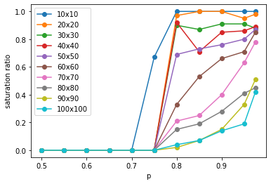
Let's stop looking at individual trajectories, and plot the saturation ratio (of the 100 trajectories), for different sized grids, at different $p$s:

This confirms what we saw on the trajectory plots:

• higher $p$ leads to higher likelihood of saturation
• higher $N$ makes it harder to saturate, ie. for a higher $N$ spin glass $p$ also has to be higher to saturate

Conclusion

The lower $N$ curves suggest that there is a critical $p$, above which trajectories are very likely to saturate. I suspect that this is the case for larger spin glasses too, but 1000 frames is not enough to see this; however, this is not clear, since the definition of a frame is $N$-dependent. Subsequent experiments to run:

• zoom in on the critical $p$ at varous spin sizes
• see if the critical "floor to ceiling" behavior is there for large $N$, at higher frame count
• as the frame count goes to infinity, would all spin glasses at all $p$s saturate eventually?