Probabilistic spin glass - Conclusion

Introduction

I wrote 5 posts on probabilistic spin glasses:

• Part I
• Part II
• Part III
• Part IV
• Part V

Here I will summarize my main findings, misses, and reflect what I still don't have a good feel for.

Motivation

My motivation for studying these systems was to discuss a toy model similar to spin glasses, but without having to introduce the Hamiltonian, so non-physicist readers can also follow along. I'm not actually sure how well this "probabilistic spin glass" resembles spin glasses studied by physicists. (I stopped being a real physicist 10+ years ago.)

The idea was to take a $N \times N$ sized spin system, ie. each cell has two states, ↑ and ↓, or 0 and 1. If each spin is indepdendent of its neighbours, then the whole system is just a list of indepdendent random variables, the geometry doesn't matter. To make it interesting, I made the spins dependent on the neighbours: for spin $s$ and neighbour $n$: $P(s=↑ | n=↑) = P(s=↓ | n=↓) = p$. So the spins align with probability $p$ and are opposite with probability $1-p$.

The questions then are:

• given $N$ and $p$, what is the probability of each possible $N \times N$ grid, of which there are $2^{N \times N}$?
• given $N$ and $p$, how do we write a Monte Carlo simulation so that each grid out of the $2^{N \times N}$ options is generated with the correct possibility?
• how do we verify our generation procedure?
• what can we say about the entropy of the grid [ensemble]?
• if we start with some grid, can we create a dynamic update rule given $N$ and $p$?
• what happens to the system if we apply the above update rule?

Symmetry

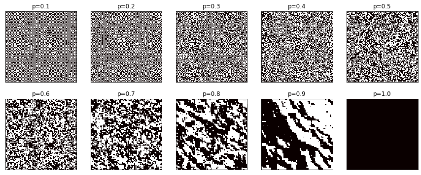
In part I, I wrote a MC method to generate grids given $N$ and $p$. They looked right, passed the smell test:

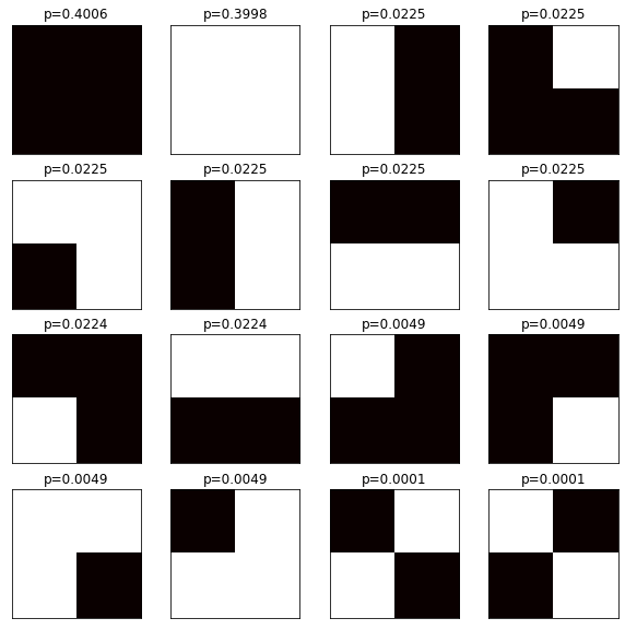
However, later I noticed that the construction method is not symmetric. Ie. there are grids that are "the same" (grid A and B are the same if you can go from one to the other by some combination of flipping all bits at once, flipping the grid up-down or left-right, or rotating the grid in either direction).

I generated a large number of grids using the (broken) method and noticed that the frequencies don't match:

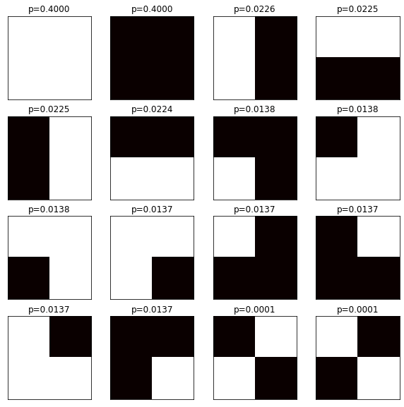
This was a pretty big miss. But, fixing this was relatively easy in the MC method, I just randomly applied a combination of the symmetry methods, and that fixed the frequencies:

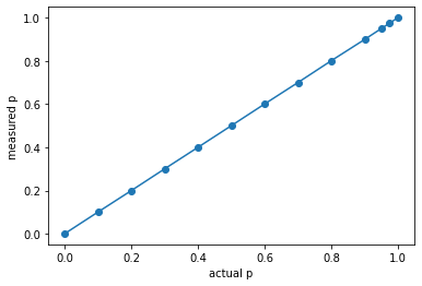
At this point I wanted to be sure, so I verified that my construction process yields the correct $p$ probabilities within the grid (it does), so I used a MC simulation to plot the calibration curve:

Direct probabilities and entropy

I also wanted to plot the entropy as it varies with $N$ and $p$. In part I, I naively used the MC method, and generated $100 \times 2^{N \times N}$ grids in the hope of getting enough samples to get meaningful frequencies. Then in part II I realized that I can just compute the direct probabilility of each possible grid, and compute the exact entropy. Interestingly, the actual plot is the same, only high probabilility configurations seem to contribute:

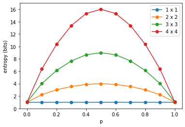
This is interesting because it's the same shape as a random coin toss (ie. a $1 \times 1$ spin glass). If somebody would ask me how to "scale up" a random coin toss to $N > 2$ outcomes, while maintaining the concave shape of the entropy curve, I would be in trouble, but this is it.

Dynamic behaviour

In part III, I wanted to see what happens if I take a spin glass (grid), and start changing the spins one-by-one, by honoring the $p$ probabililty. To see what's going on, I rendered the process as a GIF:

Naively, by looking at the evolution, I assumed that if I generate a "typical" $(N,p)$ grid, and start evolving it, it will remain "close to the original", it will remain a "typical" $(N,p)$ grid. I believe this is naive for a number of reasons:

• there are typical grids for a given $(N,p)$ because they have a relatively high probabilility, but all $2^{N \times N}$ possible grids have non-zero probability
• in the same spirit, any evolution history has non-zero probability, including the one where all spins "spontanously" go to all ↑ or all ↓, or into a nice chessboard pattern, irrespective of the current configuration. So the above assumptions, which I put into quotes, are quite wishy-washy hand-wavy, and in fact I believe they are wrong (see below).

Fraction curve

I also plotted the fraction curve in part III, this shows the majority fraction $f$ of aligned spins (whichever of there are more, ↑ or ↓). This is interesting because it shows a non-linear relationship between $p$ and $f$:

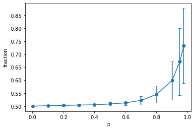
However, I completely missed this plot's $N$-dependence in part III. In part IV I realized this:

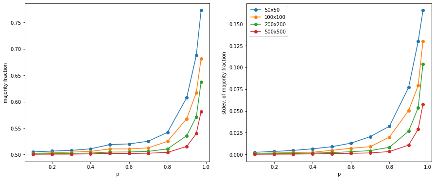
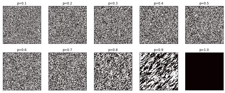
The more spins there are (the larger the grid), the harder it is (the lower the probability) for more spins to align. Essentially, as $N$ gets larger, although islands of aligned spins form, eventually by chance the islands end, and an opposite spin island forms. Since the system is very large, and both spin directions are equally favored, overall the system will have roughly equal ↑ and ↓, and from far away, it will look like random noise (like TV noise). For large $N$, $p$ has to be very close to 1 for the majority fractions to move away from 0.5! This was a major insight for me, which came quite late, in part IV.

However, it is quite obvious. For example , drawing $500 \times 500$ grids, even the high $p$ ones are close to random noise. Contrast this with the first low $N$ plots at the beginning.

Attractors

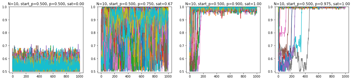
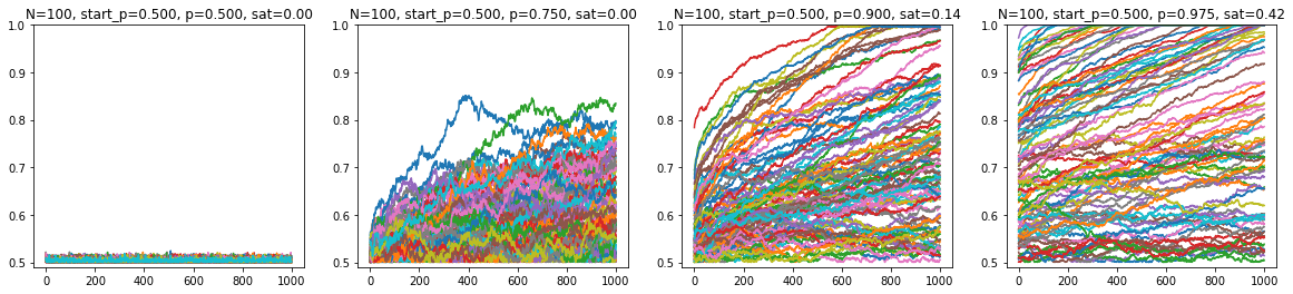
In part V, I did a more thorough, but still simulation-based, investigation of $p$ and $N$-dependence of dynamic behaviour. Plotting the saturation trajectories for the different sized grids, for different $p$s (y-axis is % of majority aligned spins, x-axis is frame/steps, each trajectory is a line, 100 lines for 100 trajectories):

$10 \times 10$:

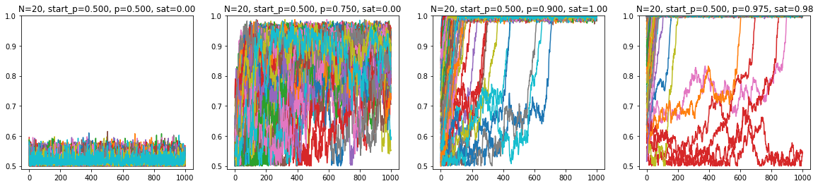
$20 \times 20$:

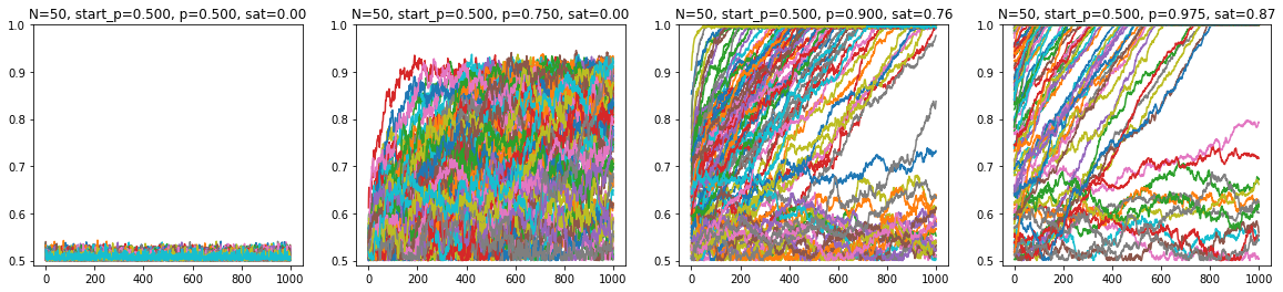
$50 \times 50$:

$100 \times 100$:

Plotting the saturation ratio (of the 100 trajectories), for different sized grids, at different $p$s:

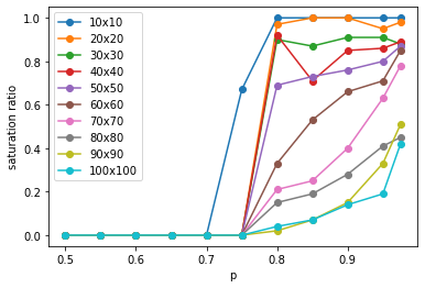
This suggests:

• higher $p$ leads to higher likelihood of saturation
• higher $N$ makes it harder to saturate, ie. for a higher $N$ spin glass $p$ also has to be higher to saturate

However, this part of the investigation is inconclusive:

• I suspect that majority fraction $f=0.5$ and $f=1$ attractors are "sticky", ie. it's hard to get away from them. For low $p$s, it's hard to get away from $f=0.5$ and it seems it practically "never" happens, then at some critical $p$ it becomes "possible" or "likely", and in those cases I believe it creeps up to $f=1$, where it gets stuck (sticky ceiling)
• as I wrote earlier, probabilistically every configuration can go into any other configuration (assuming $0 < p < 1$), but I don't know how to express the apparent stickyness of the $f$ ceiling
• it's also not clear to me whether the critical $p$, if it exists, is the same for all grid sizes, and I just have to run the simulations longer to see the same behaviour, or it differs

Conclusion

This has been an interesting investigation, purely conducted out of intellectual curiousity. I may re-visit it once I have some new ideas, especially on how to quantitatively classify the long-term dynamic behaviour and its potential attractors.