Similar posts recommendation with Doc2Vec - Part II
Marton Trencseni - Sun 04 December 2022 - machine-learning
Introduction
In the previous post, I used the Doc2Vec neural network architecture to compute the similarities between my blog posts. Using these, I am planning to add Articles You May Like recommendations to Bytepawn (this blog), based on the semantic similarity of my blog posts. In this second post I investigate the results further. The code is up on Github.
Similarity matrix
The previous post left off with showing the raw similarity matrix:
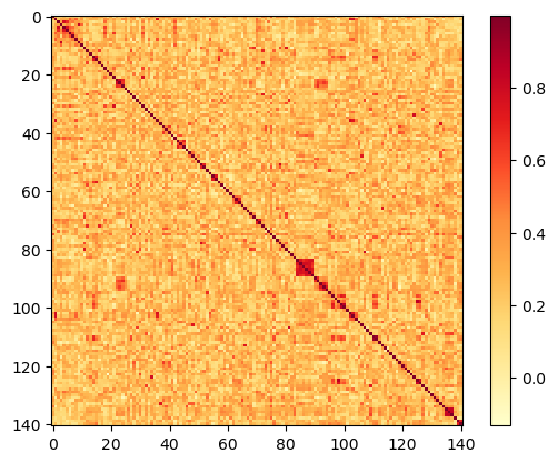
I also noted the (red) square of high similarity scores in the above plot, from id=84 to id=89. That's the cluster of articles about Probabilistic spin glasses, which all have the same filename prefix (so their integer ids are sequential, so they are sequential rows and columns in the matrix), and have very high similarity scores:
- Probabilistic spin glass - Part I
- Probabilistic spin glass - Part II
- Probabilistic spin glass - Part III
- Probabilistic spin glass - Part IV
- Probabilistic spin glass - Part V
- Probabilistic spin glass - Conclusion
Clusters
The matrix visualization doesn't work well, it only visually shows clusters that happen to be sequentially ordered, like above. We need to look at it as a graph, and find connected sub-graphs of similar articles. Plotting the entire graph is pointless, as it would have, for $N=141$ posts, $N^2=19\,881$ edges — nothing would be discernible. We need to reduce the number of edges. After some playing around, I found that keeping only similarities $ s(a, b) > 0.55 $ works well:
similarity_matrix_truncated = [[y if y > 0.55 else 0 for y in x] for x in similarity_matrix]
for i in range(len(similarity_matrix_truncated)):
    similarity_matrix_truncated[i][i] = 0
plot_matrix(similarity_matrix_truncated)
The code also zeros out the diagonal elements, to avoid plotting self-loops on the graph. First, let's see what this truncated matrix looks like as a heatmap:
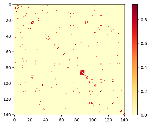
Looks promising. Now let's plot the graph:
import pandas as pd
import networkx as nx
import matplotlib.pyplot as plt

def plot_graph(m):
    labels = list(range(len(m)))
    df = pd.DataFrame(m, index=labels, columns=labels)
    G = nx.from_pandas_adjacency(df)
    plt.figure(figsize=(15, 15))
    nx.draw_networkx(G, nx.spring_layout(G), node_size=0, arrows=False, edge_color='lightgray', font_size=8)
    plt.show()

plot_graph(similarity_matrix_truncated)
Output:
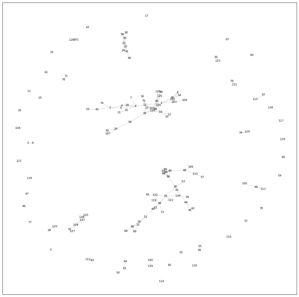
By reading off the ids for some of the clusters, we can check what they are:
print([
        [idx_lookup[63], idx_lookup[64]],
        [idx_lookup[3],  idx_lookup[9]],
        [idx_lookup[37], idx_lookup[47], idx_lookup[48], idx_lookup[106], idx_lookup[133]],
])```
Output:
[
    # good cluster, these 2 articles are about GPT-3
    [
        'how-good-a-data-scientist-is-gpt-3',
        'how-good-a-particle-physicist-is-gpt-3'
    ],
    # good cluster, these 2 articles are about A/B testing on social networks
    [
        'ab-testing-and-network-effects',
        'ab-testing-on-social-networks'
    ],
    # good cluster, these 5 articles are about entropy
    [
        'cross-entropy-joint-entropy-conditional-entropy-and-relative-entropy',
        'entropy-in-data-science',
        'entropy-of-an-ideal-gas-with-coarse-graining',
        'the-physical-sackur-tetrode-entropy-of-an-ideal-gas',
        'what-is-the-entropy-of-a-fair-coin-toss'
    ]
]
The results continue to look promising. Instead of checking these cluster manually, let's automate it:
def clusters(m):
    connected_subgraphs = set([frozenset([i]) for i in list(range(len(m)))])
    def update_subgraphs(i, j):
        join_targets = [g for g in connected_subgraphs if i in g or j in g]
        new_subgraph = frozenset({i for g in join_targets for i in g})
        for g in join_targets:
            connected_subgraphs.remove(g)
        connected_subgraphs.add(new_subgraph)
    for i in range(len(m)):
        for j in range(len(m)):
            if m[i][j] > 0:
                update_subgraphs(i, j)
    return connected_subgraphs

def print_clusters(connected_subgraphs):
    for g in connected_subgraphs:
        if len(g) == 1:
            for i in g:
                print(f'Singleton: {idx_lookup[i]}')
    for g in connected_subgraphs:
        if len(g) > 1:
            print('Cluster:')
            for i in g:
                print({idx_lookup[i]})
And now let's print them:
c = clusters(similarity_matrix_truncated)
print_clusters(c)
Output:
Singleton: understanding-facebook-planout-ab-testing-framework
Singleton: ab-tests-moving-fast-vs-being-sure
Singleton: the-culture-map
Singleton: more-data-scientists-should-learn-sql
...
Cluster:
{'aa-testing-and-false-positives-with-cuped'}
{'correlations-seasonality-lift-and-cuped'}
{'reducing-variance-in-ab-testing-with-cuped'}
{'reducing-variance-in-conversion-ab-testing-with-cuped'}
{'ab-testing-and-multi-armed-bandits'}
{'multi-armed-bandits-and-false-positives'}
{'ab-testing-and-the-historic-lift-paradox'}
{'five-ways-to-reduce-variance-in-ab-testing'}
Cluster:
{'how-good-a-particle-physicist-is-gpt-3'}
{'how-good-a-data-scientist-is-gpt-3'}
Cluster:
{'exploring-prior-beliefs-with-mcmc'}
{'food-deliveries-bayes-and-computational-statistics'}
Cluster:
{'solving-openai-gym-classic-control-problems-with-pytorch'}
{'using-simulated-self-play-to-solve-all-openai-gym-classic-control-problems-with-pytorch'}
{'solving-the-cartpole-reinforcement-learning-problem-with-pytorch'}
...
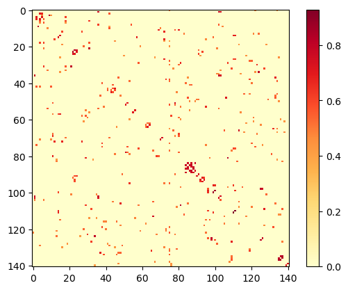
It still looks good! However, this approach isn't the most representative: many posts are left as singletons, because all their similarity weights are less than the cutoff of $ s(a, b) > 0.55 $. However, in practice the recommendation engine would still return the top $n$ for them. A better approach is to keep the top $n$ post recommendations (edge) for each post (node), irrespective of weight. Let's start with $n=3$:
# another approach, to avoid singletons:
# for each post, get the top n=3 most similar
def similarity_matrix_top_n(n=3):
    m = [[0 for _ in range(len(posts))] for _ in range(len(posts))]
    for i in list(range(len(m))):
        sp = similar_posts(i)
        idxs = [tagged_posts[p[0]][1][0] for p in sp]
        for k, j in enumerate(idxs):
            m[i][j] = sp[k][1]
    return m

similarity_matrix_truncated = similarity_matrix_top_n(n=3)
plot_matrix(similarity_matrix_truncated)
plot_graph(similarity_matrix_truncated)
The heatmap:
The graph:
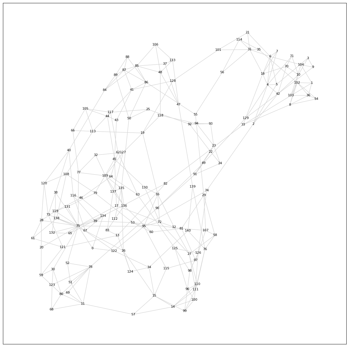
The graph is now fully connected, which makes sense. The challenge now is that it's again hard to make sense of the adjacencies. Let's re-run, but only keep the top $n=2$:
similarity_matrix_truncated = similarity_matrix_top_n(n=2)
plot_graph(similarity_matrix_truncated)
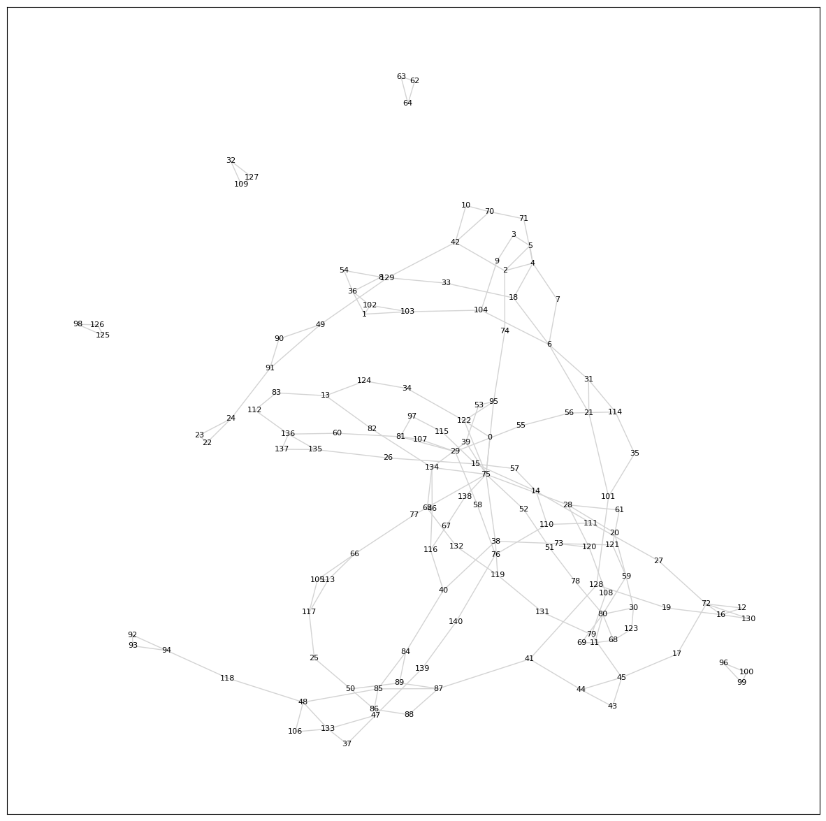
Most of the graph is still a big fully-connected cluster, let's try again with $n=1$:
similarity_matrix_truncated = similarity_matrix_top_n(n=1)
plot_graph(similarity_matrix_truncated)
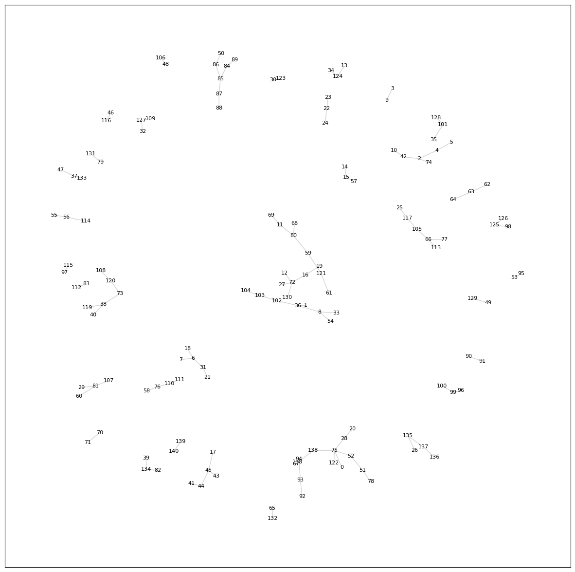
This now looks interesting. There are reasonably sized clusters, and all posts are in a cluster. Let's look at them explicitly:
c = clusters(similarity_matrix_truncated)
print_clusters(c)
Output (note that there are no singletons):
Cluster:
{'building-a-toy-python-dataclass-decorator'}
{'rxe-literate-and-composable-regular-expressions'}
{'building-a-simple-python-enum-class-part-ii'}
{'building-a-simple-python-enum-class'}
Cluster:
{'automating-a-call-center-with-machine-learning'}
{'backtraced-growth-accounting'}
{'warehouse-locations-with-kmeans'}
{'machine-learning-at-fetchr'}
{'calibration-curves-for-delivery-prediction-with-scikit-learn'}
{'arabic-name-classification-with-scikit-learn-and-pytorch'}
Cluster:
{'the-german-tank-problem-in-world-war-ii'}
{'beyond-the-central-limit-theorem'}
{'ab-testing-and-the-ttest'}
{'ab-testing-and-the-ztest'}
{'ab-testing-and-the-central-limit-theorem'}
...
Note that I'm not implying here that I would only use the top $n=1$ recommendation. This is just to see what kind of clusters are formed by the similarity scores, and whether it makes sense — it's verification.
Conclusion
The similarities look good — I see no reason to invest any more time into this part. In Part III, I will add the recommendations to the website!